Simple RNN for IMDb Sentiment Analysis
Introduction
An end-to-end deep learning project using a simple RNN. The dataset used is the IMDb dataset, which consists of movie reviews. The goal is to use the text reviews as input and predict output labels indicating whether the review is positive or negative using a simple RNN. The primary objective of this project is to implement and analyze a Simple RNN on the IMDb dataset.
The dataset contains approximately 50,000 records, which is a substantial amount for training. Let’s understand the overall architecture and workflow.
Project Architecture

The workflow begins with the input data, which is the reviews dataset. We perform feature engineering or feature transformation on this data to prepare it for ingestion into the simple RNN for training the neural network.
After preprocessing, we build the simple RNN architecture and feed the transformed data into it. Once training is complete, the model is saved as a .keras file. This format is commonly used in deep learning with Keras, similar to how pickle files are used in machine learning.
Following model training, we create a Streamlit web application for user interaction and then deploy the application to the cloud.
Key Components of Simple RNN Model
The simple RNN model consists of two important components:
- The embedding layer
- The simple RNN layer
Understanding the Embedding Layer
The embedding layer is responsible for converting words into vector representations. This is crucial because the simple RNN processes numerical vectors rather than raw text.
Since words are categorical data, they must be converted into vectors of fixed dimensions before being input to the RNN. The embedding layer performs this conversion by mapping each word to a dense vector representation.
The embedding layer uses word embeddings, which are learned representations of words in a continuous vector space. Techniques such as Word2Vec are examples of word embedding methods that can be utilized within the embedding layer.
Loading the IMDb Dataset
The IMDb dataset is available inside TensorFlow. We can load it directly from there. We will define the vocabulary size, which is the maximum number of words to consider. Then, we will load the training and testing data along with their labels.
1
2
3
4
5
6
7
max_features = 10000 # vocabulary size

(X_train,y_train),(X_test,y_test) = imdb.load_data(num_words=max_features)

# Print the shape of the data
print(f'Training data shape: {X_train.shape}, Training labels shape: {y_train.shape}')
print(f'Testing data shape: {X_test.shape}, Testing labels shape: {y_test.shape}')
Exploring the Dataset
The training and testing datasets each contain 25,000 records. Each record is a review represented as a sequence of integers, where each integer corresponds to a specific word index in the vocabulary. The labels are binary, indicating positive (1) or negative (0) sentiment.
Let’s inspect a sample review and its label.
1
2
3
4
5
sample_review=X_train[0]
sample_label=y_train[0]

print(f"Sample review (as integers):{sample_review}")
print(f'Sample label: {sample_label}')
Understanding the Integer Encoding
Each review is represented as a list of integers, where each integer is an index corresponding to a word in the vocabulary. This is a form of one-hot representation where the index represents the word. The vocabulary size is 10,000, so indices range within this limit.
Decoding the Integer Encoded Review
To understand the actual text, we need to map the integer indices back to their corresponding words. The IMDb dataset provides a word index dictionary for this purpose. We will reverse this dictionary to map indices to words and decode the sample review.
1
2
3
4
5
6
word_index = imdb.get_word_index()
reverse_word_index = {value: key for key, value in word_index.items()}

decoded_review = ' '.join([reverse_word_index.get(i - 3, '?') for i in sample_review])

print('Decoded review:', decoded_review)
I have explained why we need to do i-3 while decoding the review here.
Padding Sequences
Neural networks require inputs of uniform length. Since reviews vary in length, we apply padding to ensure all sequences have the same length. We will use the pad_sequences function from TensorFlow’s preprocessing module to pad the sequences to a maximum length of 500 words using pre-padding (adding zeros at the beginning).
1
2
3
4
5
6
max_length = 500

x_train = sequence.pad_sequences(x_train, maxlen=max_length)
x_test = sequence.pad_sequences(x_test, maxlen=max_length)

print('Padded x_train sample:', x_train[0])
Training Simple RNN with Embedding Layer
First, we initialize the model as a sequential model. The initial layer we add is an embedding layer. This layer converts words into dense vectors of fixed size, which helps the network understand the semantic relationships between words.
1
2
model = Sequential()
model.add(Embedding(input_dim=max_features, output_dim=128))
Here, max_features represents the vocabulary size, and 128 is the embedding dimension chosen for feature representation.
Next, we add a simple RNN layer with 128 neurons and use the ReLU activation function. This layer processes the sequence data and captures temporal dependencies.
1
model.add(SimpleRNN(128, activation='relu'))
Finally, we add a dense output layer with a single neuron and a sigmoid activation function, suitable for binary classification tasks.
1
model.add(Dense(1, activation='sigmoid'))
After constructing the model, we can view its summary to check the architecture.
1
model.summary()
Before training, we compile the model by specifying the optimizer, loss function, and evaluation metrics. For binary classification, we use the Adam optimizer and binary cross-entropy loss. Accuracy is used as the metric.
1
2
3
4
5
model.compile(
    optimizer='adam',
    loss='binary_crossentropy',
    metrics=['accuracy']
)
To prevent overfitting and optimize training time, we implement early stopping. This callback monitors the validation loss and stops training if it does not improve for a specified number of epochs (patience). It also restores the best weights observed during training.
1
2
3
from tensorflow.keras.callbacks import EarlyStopping

early_stopping = EarlyStopping(monitor='val_loss', patience=5, restore_best_weights=True)
We train the model using the training data, specifying the number of epochs, batch size, and validation split. We also pass the early stopping callback to halt training when appropriate.
1
2
3
4
5
history = model.fit(
    X_train, y_train, epochs=10, batch_size=32,
    validation_split=0.2,
    callbacks=[earlystopping]
)
The trained model was saved into a .keras file format. This allows for easy loading and reuse of the model later. The command used was model.save(). The model file is saved and ready for future use.
Model Prediction
A new Jupyter notebook file named Prediction.ipynb was created to handle model loading and prediction tasks.
The necessary libraries were imported, including datasets and preprocessing utilities. The IMDb dataset’s word index was loaded, along with a reverse word index to map indices back to words. The saved model file was loaded, and the model summary was displayed to review the architecture and parameters.
Exploring Model Details
The model summary provides an overview of the network architecture. Additionally, the model’s weights can be accessed using the get_weights() method, which returns all parameters used in the model. Sometimes, instead of saving the entire model as a file, the architecture and weights are saved separately and combined later.
Utility Functions for Prediction
Two helper functions were created to facilitate prediction:
- Decoding the Review: Converts encoded sequences back to readable text.
- Preprocessing Input: Encodes and pads the input text to a fixed length.
The preprocessing function uses sequence.pad_sequences with a maximum length of 500, which matches the maximum sequence length used during training the simple RNN model.
Prediction Function Implementation
The prediction function takes a review as input. It first preprocesses the review by encoding and padding it. Then, it passes the preprocessed input to the loaded model’s predict method to obtain a prediction score.
Based on the prediction score, the function determines the sentiment:
- If the prediction score is greater than 0.5, the sentiment is classified as positive.
- Otherwise, it is classified as negative.
The function returns both the sentiment label and the prediction score.
Example Prediction
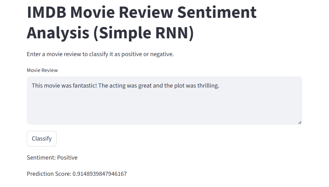
An example review was used to test the prediction function:
The movie was fantastic, the acting was great, and the plot was thrilling.
When passed through the predict_sentiment function, the output was:
- Sentiment: positive
- Prediction score: 0.91
Since the prediction score exceeds 0.5, the sentiment is correctly identified as positive.
Issues with Model Prediction
To achieve the above prediction result, a few modifications were made to the model configuration. Initially, the same review was incorrectly classified as Negative. After adjusting the model and training parameters, the prediction improved and aligned with the expected sentiment.
The following changes were implemented:
- Removed the activation function from the Embedding layer, allowing the model to use the default
tanhactivation, which is better suited for sequence modeling. - Increased the EarlyStopping patience from 5 to 8, enabling the model to continue training longer and avoid stopping prematurely before reaching better generalization.
- Extended the number of training epochs from 10 to 20, giving the model additional opportunities to learn meaningful patterns from the data.
Despite hyperparameter tuning, the model fails to achieve satisfactory accuracy and does not consistently predict the correct sentiment on unseen examples.
This highlights the inherent limitations of a Simple RNN architecture. Simple RNNs struggle to capture semantic meaning and long-term dependencies in text data due to issues such as the vanishing gradient problem, making them ineffective for understanding long or complex reviews.
Even after these updates, the model is still giving wrong sentiment predictions. Here’s an example:
This movie was bad. I don’t like it.
- Sentiment: positive
- Prediction score: 0.87
To further improve model performance, exploring advanced variants of RNNs such as LSTM or GRU would be a logical next step. However, the primary objective of this project is to implement and analyze a Simple RNN on the IMDb dataset.
With this objective achieved, we will now move to the next phase: building a Streamlit-based web application to enable user interaction and demonstrate the model’s predictions.
Streamlit Web App
The main script, main.py, will contain the code for the Streamlit app. The structure will be similar to Prediction.ipynb, including functions for decoding reviews and preprocessing text. All components will be combined, and the model will be loaded.
A text area is created for the user to input a movie review. When the classify button is clicked, the input is preprocessed and passed to the model for prediction. The result is displayed in the app as shown below.
Conclusion
This project successfully demonstrates the end-to-end implementation of a Simple RNN for sentiment analysis while clearly exposing its limitations. It serves as a strong foundational exercise for understanding why more advanced sequence models are required in modern NLP tasks.