US Emissions Analysis Dashboard using Databricks

Overview

In this project, I built an interactive United States emissions analysis dashboard using Databricks Free Edition.

The goal was to analyze real EPA emissions data and answer practical questions such as:

• Where are emissions geographically concentrated in the U.S.?
• Which states contribute the most to total emissions?
• How do emissions scale with population at the county level?
• Do highly populated areas necessarily emit more per person?

This project covers the full analytics lifecycle:

• Raw data ingestion
• Data cleaning and transformation
• SQL-based analysis
• Dashboard creation and storytelling

Project Architecture

Tech Stack

• Databricks Free Edition
• Databricks SQL
• Built-in Databricks Dashboards

Key Skills Demonstrated

• Working with raw, imperfect data
• SQL aggregations and calculations
• Handling data quality issues (numeric strings, commas)
• Geographic visualization (latitude/longitude)
• Analytical storytelling

Dataset Overview

The dataset contains ~3,000 rows but many columns, including:

• Greenhouse Gas emissions (metric tons of CO₂ equivalent)
• Population
• Latitude & Longitude
• County name
• State name and abbreviation

To keep the project focused, I selected only the fields relevant to emissions analysis and geography, rather than attempting to model every variable.

Step 1: Creating a Databricks Catalog and Table

I started by creating a dedicated catalog to keep the project organized.

CREATE CATALOG emissions;

Inside the default schema, I uploaded the raw CSV file and created a table named:

emissions.default.emissions_data

Databricks automatically inferred column types.

At this stage, no transformations were applied — the table represents raw source data, which mirrors real-world analytics workflows.

Step 2: Understanding the Business Problem

The analysis was framed to build a dashboard that answers:

• Where do emissions occur geographically?
• Which regions should be prioritized for intervention?
• How do emissions compare relative to population?

This framing guided every query and visualization decision.

Step 3: Visualizing Emissions by Location (Latitude & Longitude)

The first analysis focused on geographic distribution.

SELECT
	latitude,
	longitude,
	`GHG emissions mtons CO2e`
FROM emissions_data

I visualized the raw coordinates using a point map in Databricks.

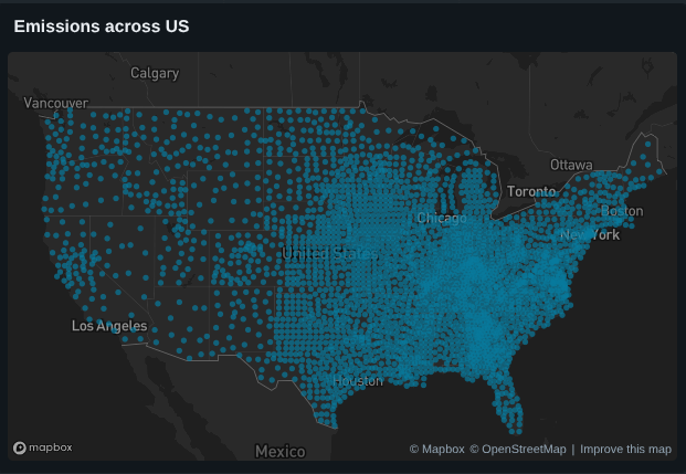
Insight

• Emissions cluster heavily in the Mid to Eastern U.S.
• The West Coast, despite high population, shows lower relative emissions

Step 4: Calculating Emissions Per Person (County Level)

This step required data cleaning, because emissions values were stored as strings with commas.

Cleaning and Calculation

SELECT
	county_state_name,
	population,
	TRY_CAST(REPLACE(`GHG emissions mtons CO2e`, ',', '') AS DOUBLE) / NULLIF(CAST(population AS DOUBLE), 0) AS emissions_per_person
FROM emissions_data
ORDER BY emissions_per_person DESC;

Step 5: Scatter Plot — Emissions vs Population

Using the cleaned data, I created a scatter plot:

• X-axis: Emissions per person
• Y-axis: Population
• Tooltip: county_state_name

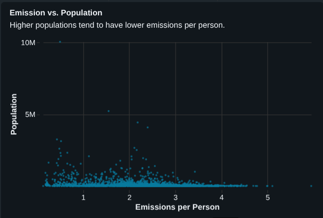
Key Findings

• Highly populated counties tend to have lower emissions per person
• Smaller counties often show disproportionately high emissions per person
• Example:
  • Los Angeles County → very high population, low emissions per person
  • Small counties in Nelson / Steele → high emissions per person

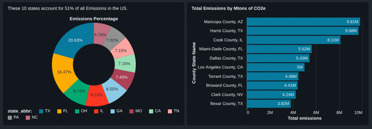
Step 6: Total Emissions by State (Top 10)

Next, I analyzed which states emit the most overall.

SELECT
	state_abbr,
	SUM(TRY_CAST(REPLACE(`GHG emissions mtons CO2e`, ',', '') AS DOUBLE)) AS total_emissions
FROM emissions_data
GROUP BY state_abbr
ORDER BY total_emissions DESC
LIMIT 10;

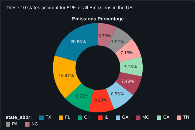
Step 7: How Much Do the Top 10 States Contribute?

To quantify impact, I calculated what percentage of total U.S. emissions comes from the top 10 states.

WITH top10 AS
(
	SELECT
		state_abbr,
		SUM(TRY_CAST(REPLACE(`GHG emissions mtons CO2e`, ',', '') AS DOUBLE)) AS total_emissions
	FROM emissions_data
	GROUP BY state_abbr
	ORDER BY total_emissions DESC
	LIMIT 10
)

SELECT
	SUM(total_emissions) AS top10_emissions,
	(SUM(total_emissions)/
	(SELECT SUM(TRY_CAST(REPLACE(`GHG emissions mtons CO2e`, ',', '') AS DOUBLE)) FROM emissions_data))*100
AS top10_emissions_percentage
FROM top10;

Result

➡ The top 10 states account for ~51% of total U.S. emissions

This single metric adds strong narrative value to the dashboard.

Step 8: Top 10 Emitting Counties

Finally, I identified counties with the highest absolute emissions.

SELECT
	county_state_name,
	population,
	TRY_CAST(REPLACE(`GHG emissions mtons CO2e`, ',', '') AS DOUBLE) AS total_emissions
FROM emissions_data
ORDER BY total_emissions DESC
LIMIT 10;

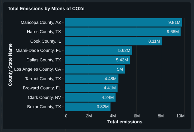
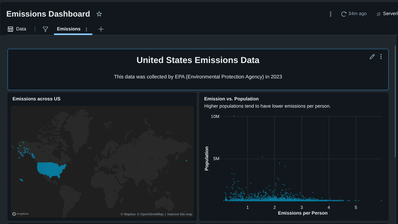
Final Dashboard Components

The completed dashboard includes:

1. Emissions map (latitude & longitude)
2. Emissions vs population scatter plot
3. Top 10 emitting states (percentage)
4. Top 10 emitting counties (absolute totals)
5. Supporting annotations and insights