Earthquake Data Engineering Project

I have successfully designed and implemented a robust, automated data engineering and analysis project leveraging the full capabilities of Microsoft Fabric, focusing on worldwide earthquake events data. This project followed the Medallion Architecture pattern, ensuring the data’s structure and quality improved incrementally across three distinct layers: Bronze, Silver, and Gold.

Project Setup

The implementation began by establishing the core environment and selecting the appropriate data source.

1. Environment Configuration (Microsoft Fabric)

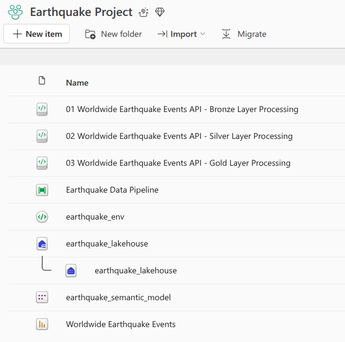
I initiated the project by creating a dedicated Workspace (named Earthquake Project). Within this workspace, I provisioned a new Lakehouse called earthquake_lakehouse. This Lakehouse functions as the central data repository, designed to store structured and unstructured data, and is optimized for large-scale storage and high-performance business intelligence (BI) analytics.

The creation of the Lakehouse automatically provided essential components:

• Lakehouse view: This provides the interface to view the data files and folders. It is divided into two parts, Tables and Files to view the data. Delta format, which provides versioned and transactional storage, was the default file format for tables within the Lakehouse.

• SQL Analytics Endpoint: This gave me an SQL-based interface to execute queries and perform data exploration directly on the data stored in the Lakehouse, using familiar SQL syntax.

2. Data Source Definition (USGS API)

The data source chosen was the USGS Earthquake Catalog API. The base URL used for accessing the data was https://earthquake.usgs.gov/fdsnws/event/1/[METHOD[?PARAMETERS]].

I utilized the query method to submit data requests, allowing me to specify parameters such as time boundaries and magnitude characteristics. Critical implementation decisions based on the API documentation included:

• Format Selection: Although the default output format is quakeml, I specified format=geojson because this format is supported by the query method and is necessary for extracting structured geometric data and detailed event properties.

• Time Parameters: I relied on the starttime and endtime parameters to limit events to a specific period. All times use the ISO8601 Date/Time format, with UTC assumed if no timezone is specified. For example, specifying only the date (e.g., 2026-01-04) implies the time is the start of that day (00:00:00).

• Result Limits: I was aware that the service limits queries to 20,000 events, and exceeding this generates a “400 Bad Request” HTTP response.

Step 1: Bronze Layer Processing (Notebook 01)

The Bronze layer pipeline was implemented in Notebook 01, focusing on ingesting raw data with minimal modification.

1. Data Fetching and Validation: I used the Python requests library within the Fabric notebook to execute the API call. The URL string was formatted to dynamically accept start_date and end_date variables, allowing for programmatic data retrieval for any specific time period. I validated the request success by checking for an HTTP status code of 200.
2. Raw Data Extraction: Upon successful retrieval, I accessed the relevant earthquake information by parsing the JSON response and extracting the data associated with the features key,. This raw data contained nested objects, including the geometry (coordinates) and the properties (magnitude, time, significance, etc.).
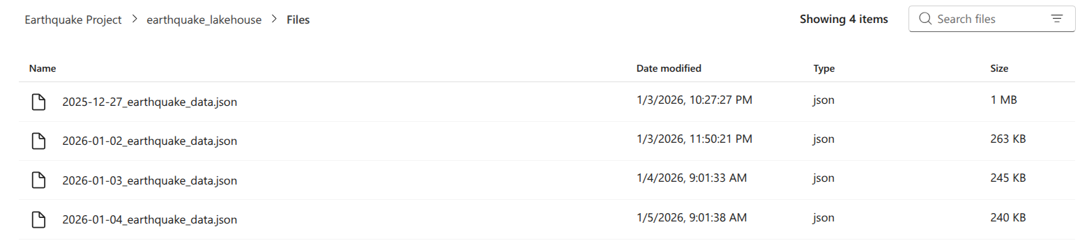
3. Storage Mechanism: The extracted raw JSON data was stored in the Lakehouse files section. The file path was constructed using the pattern Lakehouse default.files/[start_date]_earthquake_data.json. Using the start_date as a prefix ensured that when running the ingestion process daily, new data would be written to a unique file, preventing overwriting and aiding data retention. I used the json.dump method with the mode set to write (w) to handle the file writing.

Files in bronze layer:

Step 2: Silver Layer Processing (Notebook 02)

Notebook 02 handled the Silver layer processing, transforming the raw JSON into a structured Delta table format, focusing on cleansing and consolidation.

1. Data Ingestion and PySpark Setup: I read the raw JSON file from the Bronze layer (using the dynamic start_date parameter) into a PySpark DataFrame,.
2. Structural Flattening: The key transformation here involved converting the nested JSON fields into discrete, accessible columns.
   • Geometry Extraction: The geometry.coordinates field was an array of three elements: longitude, latitude, and elevation,. I extracted these elements using the PySpark get_item method with specific indexing: index 0 for longitude, index 1 for latitude, and index 2 for elevation.
   • Properties Extraction: I extracted necessary attributes like title, mag, sig, time, and updated directly from the properties column using dot notation (e.g., properties.mag).
3. Time Data Transformation: The time and updated columns were initially provided in Unix timestamp milliseconds format. To convert these to a standard timestamp format, I performed a two-step transformation:
   • The values were divided by 1,000 to convert milliseconds into seconds.
   • The result was then explicitly cast as the TimestampType.
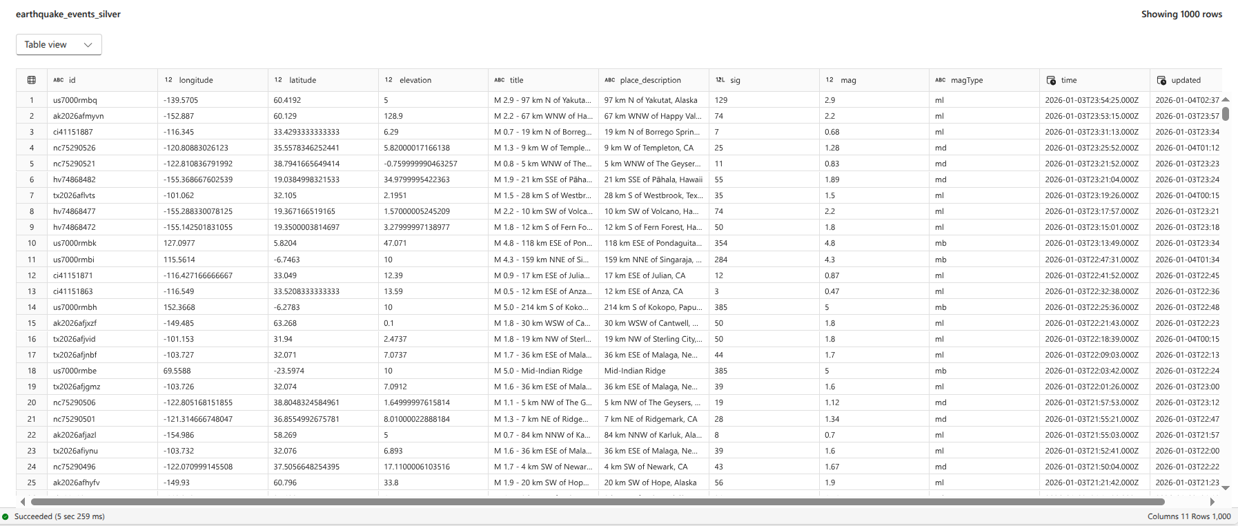
4. Storage: The cleansed and structured data was written/appended to a Delta table named earthquake events silver in the Lakehouse. This Delta table format provides transactional capabilities, facilitating efficient data appending for subsequent daily processes.

Final table in silver layer:

Step 3: Gold Layer Processing (Notebook 03)

The Gold layer refined the data for specific BI consumption by adding business-ready attributes and logic.

1. Environment Setup for Enrichment: To perform geo-enrichment, I needed the external Python library reverse_geocoder. Since this is not a built-in library, I created a custom Microsoft Fabric Environment (earthquake_env). I installed the reverse_geocoder library via PyPI within this new environment and published it, waiting for the publishing to succeed before proceeding.
2. Geo-Enrichment Implementation (Country Code):
   • I defined a Python function (get_country_code) that accepts latitude and longitude coordinates as input tuples. This function used the reverse_geocoder.search method to identify the location details.
   • I registered this function as a Spark User Defined Function (UDF) to allow its execution across the PySpark DataFrame.
   • The UDF was invoked to create a new column, country_code, which retrieved the ISO 2-digit country code (CC) for each event based on its coordinates,.
3. Business Classification: I applied conditional logic to categorize the events based on the sig (significance) attribute. This created the column sig_class:
   • Low: If significance was less than 100.
   • Moderate: If significance was greater than or equal to 100 but less than 500.
   • High: If significance was 500 or greater.
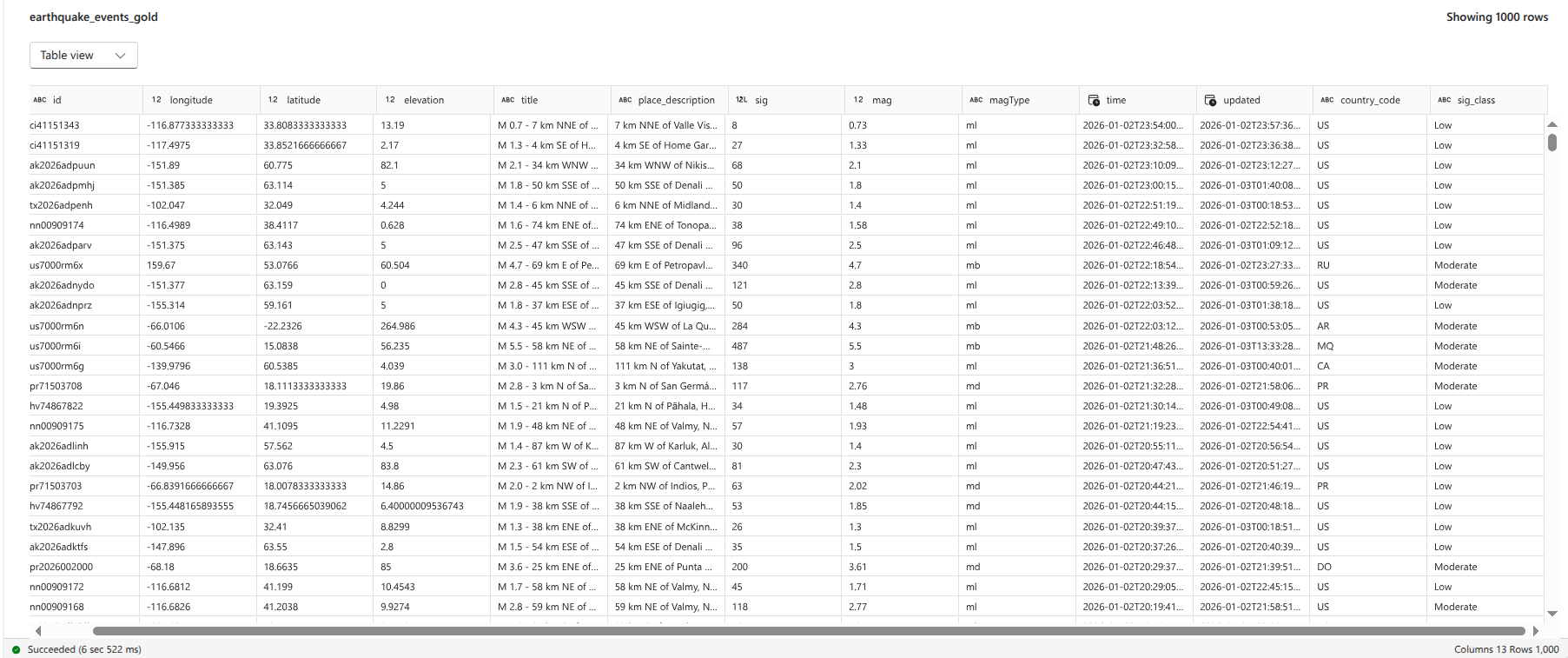
4. Storage: The final, enriched DataFrame was appended to the Delta table earthquake_events_gold, making it the definitive source for BI reporting. In the final implementation, the notebook included logic to filter the Silver table for records occurring after the received start_date parameter to prevent reprocessing duplicate data during subsequent runs.

Final table in gold layer:

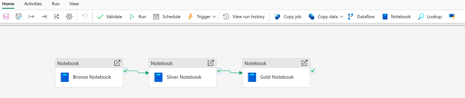
Step 4: Pipeline Orchestration (Data Factory)

I created a Data Factory pipeline named Earthquake Data Pipeline to automate the sequential execution of the created notebooks.

1. Notebook Task Chaining: The pipeline comprised three chained Notebook tasks (Bronze $\rightarrow$ Silver $\rightarrow$ Gold), linked using the “On Success” dependency to ensure they run sequentially,.
2. Dynamic Parameterization: The pipeline was responsible for dynamically calculating and passing the start_date and end_date parameters into the notebooks. This was necessary for daily scheduling.

• start_date Calculation (Yesterday): I used a combination of dynamic functions: FormatDateTime(AddDays(UTCNow(), -1), 'yyyy-MM-dd'). This expression first retrieves the current UTC time (UTCNow), subtracts one day (AddDays), and formats the result into the required YYYY-MM-DD string format.

@formatDateTime(adddays(utcNow(), -1), 'yyyy-MM-dd')

• end_date Calculation (Today): I used FormatDateTime(UTCNow(), 'yyyy-MM-dd'). This provided the current date, ensuring data was fetched up to the start of the current day.

@formatDateTime(utcNow(), 'yyyy-MM-dd')

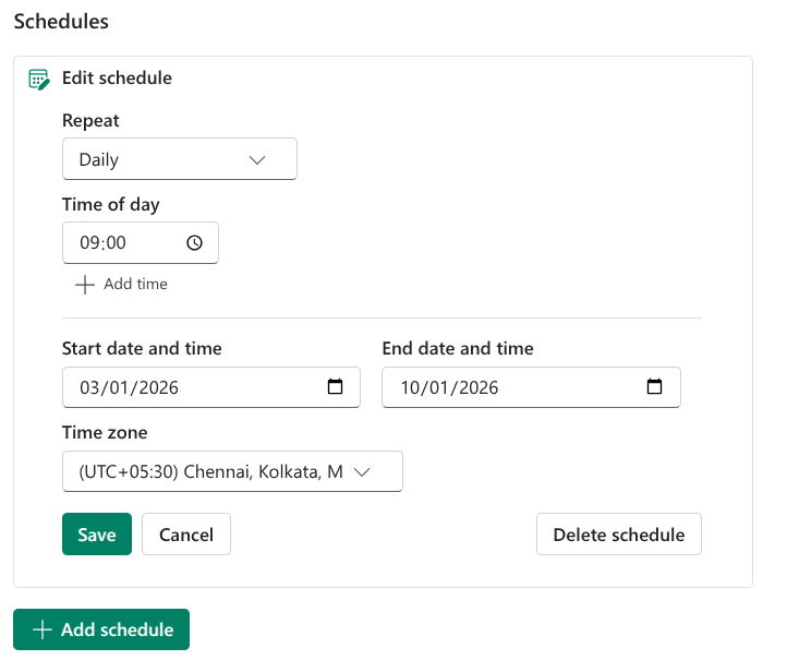
1. Automation: By defining these dynamic parameters and chaining the tasks, I established a complete ETL workflow that could be scheduled to run daily, automating the ingestion and refinement of new earthquake data.

Schedule:

Overall pipeline:

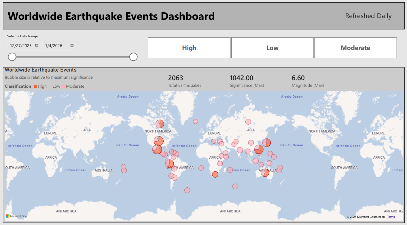
Step 5: Business Intelligence Reporting (Power BI)

The final step involved creating a Power BI report using the Gold layer data, enabling high-performance visualization.

1. Direct Lake Connection: I utilized the Direct Lake mode to connect Power BI to the Lakehouse’s semantic model. This provided a “fast path” connection, loading data directly from the Lakehouse into the Power BI engine without requiring data import or duplication, maximizing analytical speed.
2. Semantic Model Creation: I accessed the SQL Endpoint’s reporting tab to create the semantic model, ensuring the refined earthquake_events_gold table was added to the model for reporting access.
3. Report Visual Design:
   • Map Visual: I ensured the map and field map visuals setting was enabled in the Fabric Admin tenant settings. The map used the country_code for location. The bubble size was determined by the maximum significance recorded for that location, and the color legend was driven by the categorical sig_class (Low, Moderate, High).
   • Tooltips and Metrics: I enhanced tooltips by aggregating the event ID field using the count function, renaming it to Number of Events, alongside displaying the maximum significance. I also added Card visuals to display key metrics like the total number of earthquakes and the maximum significance observed.
   • Interactivity: I included slicers based on the time column (allowing selection of a date range) and the sig_class (formatted as tiles) to enable dynamic filtering and analysis.

Final Power BI report:

Final Workspace files:

All notebooks are available in my GitHub repository of this project.

Conclusion

This implementation successfully transformed raw, complex API data into a high-value, organized, and easily digestible business intelligence report which is scheduled to refresh daily, demonstrating my proficiency across the core Data Engineering, Data Factory, and Power BI experiences within Microsoft Fabric.